Reads in Two Polynomials at a Time With Coefficient and Exponent From a File

What Are Polynomials?

A polynomial is an expression containing constants and variables connected only through basic operations of algebra.

Learning Objectives

Describe what polynomials are and their defining characteristics

Cardinal Takeaways

Cardinal Points

• A polynomial is a finite expression constructed from variables and constants, using the operations of addition, subtraction, multiplication, and taking non-negative integer powers.
• A polynomial tin be written equally the sum of a finite number of terms. Each term consists of the product of a constant (chosen the coefficient of the term) and a finite number of variables (usually represented past messages) raised to integer powers.

Key Terms

• polynomial: an expression consisting of a sum of a finite number of terms, each term beingness the product of a abiding coefficient and one or more variables raised to a non-negative integer power, such as [latex]a_n x^due north + a_{n-1}x^{n-1} +… + a_0 x^0[/latex].
• degree: the sum of the exponents of a term; the society of a polynomial.
• coefficient: a abiding by which an algebraic term is multiplied.

Polynomials are widely used algebraic objects. They have the form of a sum of scaled powers of a variable.

Monomials over [latex]\mathbb{R}[/latex]

Let [latex]\mathbb{R}[/latex] be the set of real numbers. A monomial over [latex]\mathbb{R}[/latex] in a single variable [latex]x[/latex] consists of a non-negative ability of [latex]x[/latex], multiplied with a nonzero constant [latex]c \in \mathbb{R}.[/latex] So a polynomial looks like

[latex]cx^north[/latex],

where [latex]due north \geq 0[/latex] is an integer and [latex]c \not = 0[/latex] is a real number. If we want to give the polynomial a proper noun, say [latex]M[/latex], nosotros denote that its variable is [latex]ten[/latex] by writing [latex]ten[/latex] between brackets:

[latex]1000(x)=cx^n[/latex].

The exponent [latex]northward[/latex] is called the caste of [latex]M(x).[/latex] The constant [latex]c[/latex] is the coefficient.

Examples

[latex]\sqrt{2}x^7[/latex]is a monomial of degree 7 and coefficient [latex]\sqrt{2}[/latex].

[latex]7x^{\sqrt{two}}[/latex], [latex]\sqrt{2}ten^{-vii}[/latex] and [latex]2x^vii - 7x^two[/latex]are not monomials. The first and the second do not accept a non-negative integer exponent and the third is a sum of two monomials.

Polynomials over [latex]\mathbb{R}[/latex]

A polynomial over [latex]\mathbb{R}[/latex] is a finite sum of monomials over [latex]\mathbb{R}[/latex]. For example

[latex]P(x)= 4x^{13} +3x^ii-\pi ten + 1[/latex]

is the finite sum of the [latex]4[/latex] monomials: [latex]4x^{thirteen}, 3x^2, -\pi 10[/latex] and [latex]1 = 1x^0.[/latex]

Information technology is likewise the sum of the 6 monomials: [latex]one/3 x^{100}, -1/3 x^{100}, 4x^{13}, 3x^ii, -\pi ten[/latex] and [latex]i[/latex], equally will be explained in the discussion about addition and subtraction of polynomials. However, we can only write down [latex]P(x)[/latex] as the sum of monomials of distinct degree in exactly one fashion, namely the first we mentioned. These monomials are called the terms of [latex]P(x).[/latex]The coefficients of [latex]P(x)[/latex] are the coefficients corresponding to its terms.

Every monomial is also a polynomial, as information technology tin can be written as a sum with one term, itself.

A special example of a polynomial is the zippo polynomial

[latex]Z(x) = 0,[/latex]

which is a sum of [latex]0[/latex] monomials.

The degree of a polynomial [latex]Q(x)[/latex] is the highest degree of one of its terms. For example, the degree of [latex]P(x)[/latex] is [latex]thirteen[/latex].

The degree of the zippo polynomial is defined to exist [latex]-\infty[/latex].

Actress: Polynomials Over Full general Rings

This function is for the interested reader only. Virtually students can skip this part, or just remember that polynomials over [latex]\mathbb{C}[/latex] are the same as polynomials over [latex]\mathbb{R}[/latex], but with complex coefficients and that the degree of a monomial in more variables equals the sum of the exponents.

We have discussed polynomials over [latex]\mathbb{R}[/latex]. Nosotros shall later encounter that we tin can add, subtract and multiply these polynomials. In general, our coefficients [latex]c[/latex] practice not need to vest to [latex]\mathbb{R}[/latex], but they can belong to any set of "numbers" in which we tin add together, subtract and multiply. These sets are called rings. Examples of rings are the real numbers [latex]\mathbb{R}[/latex], the integers [latex]\mathbb{Z}[/latex] and the circuitous numbers [latex]\mathbb{C}[/latex]. In this case, nosotros talk about complex polynomials, or polynomials over [latex]\mathbb{C}[/latex]. The caste of a polynomial is defined in the same way equally in the real case.

In particular, the polynomials over [latex]\mathbb{R}[/latex] form a band, which we denote by [latex]\mathbb{R}[x][/latex]. The polynomials over this ring will be polynomials in two variables [latex]x[/latex] and [latex]y[/latex] over [latex]\mathbb{R}[/latex].

Hither the degree in [latex]x[/latex] of [latex]ten^3y^five[/latex]is [latex]3[/latex], the degree in [latex]y[/latex] of [latex]x^3y^five[/latex]is [latex]5[/latex] and its articulation degree or caste is [latex]8[/latex].

Adding and Subtracting Polynomials

Polynomials can exist added or subtracted past combining like terms.

Learning Objectives

Explain how to add and decrease polynomials and what it means to do so

Fundamental Takeaways

Key Points

• The rules for adding and subtracting algebraic expressions employ to polynomials; merely like terms can be combined.
• Whatever two polynomials can exist added or subtracted, regardless of the number of terms in each, or the degrees of the polynomials.
• The sum or divergence of ii polynomials will have the same degree as the polynomial with the higher degree in the trouble.

Key Terms

• Commutative Holding: States that changing the club of numbers being added does not modify the result.
• caste of a polynomial: The highest value of an exponent placed on a variable in any of the terms of a polynomial.

Polynomials are algebraic expressions that contain terms that are constructed from variables and constants. Call up the rules for adding and subtracting algebraic expressions, which state that merely similar terms can exist combined.

Like terms are those that are either both constants or accept the aforementioned variables with the same exponents. For example, [latex]4x^three[/latex] and [latex]x^3[/latex]are like terms; [latex]21[/latex] and [latex]82[/latex] are also like terms. Adding and subtracting polynomials is every bit unproblematic as adding and subtracting like terms. When adding polynomials, the commutative property allows us to rearrange the terms to group similar terms together.

Note that any two polynomials can be added or subtracted, regardless of the number of terms in each, or the degrees of the polynomials. The resulting polynomial will accept the same degree as the polynomial with the higher degree in the problem.

You may be asked to add or decrease polynomials that accept terms of different degrees. For example, one polynomial may have the term [latex]x^2[/latex], while the other polynomial has no like term. If whatever term does not have a like term in the other polynomial, it does not need to be combined with any other term. It is simply carried down, with add-on or subtraction applied appropriately. Run into the second case below for a sit-in of this concept.

Example ane

Discover the sum of [latex]4x^ii - 5x + 1[/latex] and [latex]3x^2 - 8x - ix[/latex].

Outset, group similar terms together:

[latex](4x^2 +3x^2 ) + (- 5x-8x) + (1 - nine)[/latex]

Combine the like terms for the solution:

[latex]7x^2 - 13x - 8[/latex]

Example 2

Subtract: [latex](5x^3 + x^2 + ix) - (4x^2 + 7x -3)[/latex]

Start by group like terms. Remember to apply subtraction to each term in the second polynomial. Note that the term [latex]5x^iii[/latex] in the first polynomial does not have a like term; neither does [latex]7x[/latex] in the second polynomial. These are only carried down.

[latex]5x^iii + (x^two - 4x^2) + (- 7x) + (ix - (-iii)) \\ 5x^three + (x^2 - 4x^2) - 7x +(9 + three)[/latex]

Now combine the like terms:

[latex]5x^3 - 3x^2 - 7x + 12[/latex]

Discover that the reply is a polynomial of caste 3; this is also the highest caste of a polynomial in the problem.

Multiplying Polynomials

To multiply two polynomials together, multiply every term of one polynomial by every term of the other polynomial.

Learning Objectives

Explain how to multiply polynomials using the distributive property and describe the results of doing and so

Key Takeaways

Key Points

• To multiply a polynomial by a monomial, multiply every term of the polynomial by the monomial and and so add the resulting products together.
• To multiply 2 polynomials together, multiply every term of i polynomial by every term of the other polynomial.
• The caste of a product of two polynomials equals the sum of the degrees of said polynomials.
• The zeros of a product of 2 polynomial are the zeros of the two factors, combined.

Key Terms

• monomial: An algebraic expression consisting of one term.
• commutative: A binary performance is commutative if changing the order of the operands does not modify the result, for example add-on and multiplication.
• polynomial: an expression consisting of a sum of a finite number of terms, each term being the product of a abiding coefficient and 1 or more than variables raised to a non-negative integer ability, such every bit [latex]a_n 10^n + a_{northward-1}x^{n-i} +… + a_0 10^0[/latex]. Importantly, considering all exponents are positive, it is impossible to dissever past [latex]x[/latex].

Multiplying a polynomial by a monomial is a straight awarding of the distributive and associative properties. Recall that the distributive property says that

[latex]a(b + c) = ab + air-conditioning[/latex]

for all existent numbers [latex]a,b[/latex] and [latex]c.[/latex] The associative holding says that

[latex](ab)c=a(bc)[/latex]

for all real numbers [latex]a,b[/latex] and [latex]c.[/latex]

As we will treat variables in the same way as real numbers, the aforementioned backdrop hold whenever [latex]a,b[/latex] and/or [latex]c[/latex] is a variable. So for the multiplication of a monomial with a polynomial we get the following procedure:

Multiply every term of the polynomial by the monomial and so add together the resulting products together.

For example,

[latex]\brainstorm{align} 3x^two(4x-\pi)&=3x^two \cdot 4x-3x^2 \cdot \pi \\&=12x^3-3\pi ten^ii. \terminate{align}[/latex]

To multiply a polynomial [latex]P(10) = M_1(ten) + M_2(ten) + \ldots + M_n(x)[/latex] with a polynomial [latex]Q(x) = N_1(x) + N_2(x) + \ldots + N_k(ten)[/latex], where both are written equally a sum of monomials of distinct degrees, we become

[latex]\begin{align} P(x)Q(x) &= (M_1(x)+M_2(x)+ \ldots + M_n(x))Q(10) \\ &=M_1(10)Q(x) + M_2(x)Q(10) + \ldots + M_n(x)Q(x) \\ &=M_1(ten)N_1(x) + \ldots + M_1(x)N_k(10) + \ldots \\ &+M_n(x)N_1(x) + \ldots + M_n(x)N_k(x) \end{align}[/latex]

and we see that this equals the sum of the products of the terms, where every term of [latex]P(x)[/latex] is multiplied exactly once with every term of [latex]Q(10)[/latex]. Notice that since the highest degree term of [latex]P(ten)[/latex] is multiplied with the highest degree term of [latex]Q(x)[/latex] we have that the degree of the product equals the sum of the degrees, since

[latex]a^na^m=a^{1000+n}[/latex]

for all real numbers (and variables) [latex]a[/latex] and all non-negative integers [latex]thou[/latex] and [latex]n[/latex].

For convenience, we volition utilize the commutative property of addition to write the expression so that we start with the terms containing [latex]M_1(x)[/latex] and end with the terms containing [latex]M_n(x)[/latex].

This method is commonly called the FOIL method, where nosotros multiply the First, Outside, Within, and Last pairs in the expression, and so add the products of like terms together.

For example, to discover the product of [latex](2x+iii)(ten−4)[/latex], use FOIL and and so add the products together:

[latex]\begin {align} 2x \cdot ten+2x \cdot (−iv)+3 \cdot x+three \cdot(−4)&=2x^2-8x+3x-12 \\ &=2x^2−5x-12 \terminate {align}[/latex]

Zeros of a Product of Polynomials

Since nosotros made certain that the production of polynomials abides the aforementioned laws as if the variables were real numbers, the evaluation of a product of two polynomials in a given point will be the same as the product of the evaluations of the polynomials:

[latex]P(x_0)Q(x_0) = PQ(x_0)[/latex]

for all real numbers [latex]x_0.[/latex]

In particular [latex]PQ(x_0) = 0[/latex] if and only if [latex]P(x_0)Q(x_0)=0[/latex], if and only if [latex]P(x_0) = 0[/latex] or [latex]Q(x_0) = 0[/latex]. So the roots of a product of polynomials are exactly the roots of its factors, i.e. [latex]x_0[/latex] is a aught for [latex]PQ(ten)[/latex] if it is a cypher for [latex]P(x)[/latex] or for [latex]Q(10)[/latex] (and perchance both).

Polynomial and Rational Functions equally Models

Functions are unremarkably used in plumbing fixtures data to a trend line. Polynomial and rational functions are both relatively accurate and easy to apply.

Learning Objectives

Talk over the advantages and disadvantages of using polynomial and rational functions as models

Key Takeaways

Cardinal Points

• Researchers will often collect many detached samples of data, relating 2 or more than variables, without knowing the mathematical relationship betwixt them. Curve plumbing fixtures is used to create trend lines intended to fill in the points between and beyond collected data points.
• Polynomial functions are like shooting fish in a barrel to use for modeling, but sick-suited to modeling asymptotes and some functional forms, and they tin can become very inaccurate outside the bounds of the collected data.
• Rational functions can take on a much greater range of shapes and are more than authentic both inside and outside the limits of collected information than polynomial functions. Nevertheless, rational functions are more difficult to use and can include undesirable asymptotes.

Key Terms

• asymptote: A line that a bend approaches arbitrarily closely, every bit they get to infinity; the limit of the bend, its tangent "at infinity".

For a set of data containing two (or more) quantitative properties, statisticians utilise functions to denote a human relationship between ii or more distinct properties. When we find a function that lies reasonably close to the collected information points, we create a trend line which says how one property behaves every bit a function of the other ones. Nosotros call this curve fitting. Then we tin use this to make predictions almost the former property once we know something most the others.

For example, if you mensurate the pinnacle of [latex]99[/latex] 10-year olds, and you measure out how far they can bound and how fast they can run, you might be able to predict how fast the [latex]100th[/latex] child can run, only by watching them jump. Of form, this is just possible if the two quantities are related: How many uncles a kid has got has probably nothing to do with how far they can jump.

Polynomial and rational functions are piece of cake to work with because y'all only demand to make employ of elementary operations.

Recall that a polynomial part has the following form:

[latex]y=a_nx^north+a_{north-i}10^{n-i}+…+a_2x^2+a_1x+a_0[/latex]

where [latex]due north[/latex] (the caste of the polynomial) is an integer greater than or equal to [latex]0[/latex], [latex]x[/latex] and [latex]y[/latex] are variables, and [latex]0\not=a_n,a_{n-1},\ldots,a_2, a_1[/latex] and [latex]a_0[/latex] are constants.

Polynomial functions are very elementary in form and piece of cake to use, but they have limitations with regard to statistical modeling. They tin take on merely a express number of shapes and are particularly sick-suited to modeling asymptotes. They are finite when [latex]10[/latex] is finite and space when [latex]x[/latex] is space. It is especially hard to say something about the value of [latex]y[/latex] when [latex]x[/latex] is a lot bigger (smaller) than the greatest (smallest) [latex]10[/latex] in the dataset.

This need non exist a problem. For lots of datasets, their are no asymptotes and data is more or less bounded. (For example, in that location are no humans who are [latex]-10[/latex] or [latex]10000[/latex] years old.)

Polynomials have also lots of advantages:

• They are well studied: a lot of their backdrop are known.
• They are easy to compute, using only multiplication and improver.
• They are closed under rescaling or irresolute of locations: if we change a kilometer to a mile nosotros withal go a polynomial.

To deal with the asymptotic problems of polynomials, we also use rational functions:

A rational part is the ratio of two polynomial functions and has the following form:

[latex]y=\frac{a_nx^n+a_{n-i}+x^{n-one}+…+a_2x^2+a_1x+a_0}{b_mx^chiliad+b_{m-1}+x^{thousand-1}+…+b_2x^two+b_1x+b_0}[/latex]

Here, n and thou ascertain the degrees of the numerator and denominator, respectively, and together, they define the caste of the polynomial. For example, if [latex]n=ii[/latex] and [latex]yard=ane[/latex], the office is described as a quadratic/linear rational function.

Rational functions are a little more than circuitous in class than polynomial functions, just they have an reward in that they tin have on a much greater range of shapes and can effectively model asymptotes. They are besides more accurate than polynomial functions both inside and outside the limits of collected data. Withal, rational functions sometimes include undesirable asymptotes that can disrupt an otherwise smooth trend line. They are besides a lilliputian bit more difficult to compute, since you as well demand division to compute them. Nevertheless, they still run fast.

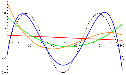
Curve fitting: Polynomial curves generated to fit points (black dots) of a sine office: The red line is a first degree polynomial; the green is a second degree; the orangish is a third caste; and the blue is a fourth degree.

Polynomials and rational functions are used for approximation in many everyday devices. For instance, every fourth dimension we have a picture show with a smartphone, our phone looks at some data points and fills in the appropriate colors in the blanks, thus saving us a lot of retention, with the help of rational functions. Every time we say something through the phone, our phone tries to reduce the groundwork racket by approximating our audio for short periods of fourth dimension, again with the help of rational functions.

howehaustrand.blogspot.com

Source: https://courses.lumenlearning.com/boundless-algebra/chapter/introduction-to-polynomials/

Share this post